GeoLab's Math Models
By Dr. Robin Steeves
Introduction
The least squares adjustment of a surveying network or traverse requires that mathematical models be used to define the relationships of the measurements made in that network to the coordinates of the stations and other optional "auxiliary" parameters.
For example, a simple 2D plane mathematical model that relates a distance measurement to the coordinates of the two points between which that distance is measured could be defined as follows (where x and y are plane coordinates, and s is a measured distance):

Basically then, the mathematical models define how the measurements can be calculated from the coordinates (and optional auxiliary parameters). We can then use these models to calculate the coordinates from the measurements in a network adjustment. The above simple 2D model for distances is not used by GeoLab because it is only an approximate model. As the distance between points becomes larger, this model becomes inaccurate.
Mathematical Models and Matrix Solutions
Please note that this article describes GeoLab's mathematical models that relate the measurements made in a survey to the coordinate and auxiliary parameters we wish to solve for in a network adjustment. A related consideration in the design of a professional level least squares adjustment software package such as GeoLab is the method used to solve the resulting system of matrix equations required by the adjustment calculations. A great deal of research has been carried out over the last 50 or so years in this branch of mathematics, and GeoLab has been designed to especially take advantage of the results of that research as applied to correctly solving surveying and geodetic network adjustments (I have performed research myself in this very interesting subject). Several methods of solving matrix equations, such as the Cholesky method, QR factorization, Householder transformations, etc, have been developed, and each is appropriate for various types of problems. Based on all the research done, GeoLab uses the efficient and stable "Block Cholesky" method to solve network matrix equations. This method has been shown to be very stable and accurate, and it takes full advantage of the positive definite normal equations resulting from a surveying or geodetic network or traverse. To further optimize the matrix solution, GeoLab also uses a proven parameter reordering method (the reverse Cutchill-McKee method).
All mathematical models used by GeoLab are geometrically rigorous (exact, with no approximations), with the exception of the observation equations for distances and azimuths on a reference ellipsoid, which should be avoided for the most accurate work. The extent of your network can be global and GeoLab's models are still exact. This article summarizes the mathematical models used in GeoLab, and explains why they are geometrically exact and preferable in the context of simpler models used by other less accurate software packages.
Historically, mathematical models used for network adjustments were formulated either on a plane or on the surface of a reference ellipsoid. To account for the fact that our measurements are made on, or near, Earth's surface, these older mathematical models required that we "reduce" our measurements to the surface of either a reference ellipsoid or a map projection plane.

As we can visualize in the simple diagram of the four reference surfaces, measurements between two points 1 and 2 on the Earth's surface will not be the same as the corresponding reduced measurements on either the map projection plane or the surface of the reference ellipsoid.
Approximate formulas were developed to make these reductions so that so-called "simpler" 2D mathematical models could then be used for network computations.
Examples of reductions that were required in the older models are such things as the Earth curvature correction, the skew normal correction, and the Laplace correction for azimuths. In the 3D model used by GeoLab, these corrections are not required because the model itself inherently contains all of this information.
So, the classical method of adjusting horizontal geodetic networks involved the reduction of measured distances, directions, angles, and azimuths to an adopted reference ellipsoid or map projection plane. This was done so that network computations could be done on a simpler 2D surface.
However, with the advent of 3D measurements such as GPS, along with the development of 3D mathematical models, the apparent advantages of the older 2D mathematical models disappeared. Not only are the 3D models more accurate, they are simpler both conceptually and computationally.
In the case where we have a mixture of GPS and conventional (angle, distance, azimuth, and leveled elevation difference) measurements, any (non-GPS) station with no measurement information for the height of that station, the height coordinate can be held fixed in the adjustment. With the 3D mathematical models, we can just as easily calculate the coordinates of the station markers themselves and not the corresponding coordinates of the projection of that point on a reference ellipsoid or map projection plane.
As our measurements become more and more accurate, and as the value of surveyed property increases, the apparent advantages of a seemingly simpler 2D mathematical model do not make sense any longer. The 3D models do not use any approximations, and they are simpler. There is therefore no need to compromise accuracy for simplicity as was done in the past.
In the remainder of this article, we will give a brief summary of the 3D mathematical models used in GeoLab. For all the details of these models and their development, please see the paper "Mathematical Models for Use in the Readjustment of the North American Geodetic Networks" by Robin R. Steeves, Technical Report Number 1, Geodetic Survey of Canada - a PDF version of this paper, “Math Models 1984.pdf” , is provided on our "Papers" page.
The 3D Coordinate Systems
Before discussing the 3D mathematical models used by GeoLab, it will be helpful to review some of the 3D coordinate system fundamentals. The following coordinate systems, all described below, are:
The Conventional Terrestrial System;
The Local Astronomic System;
The Local Geodetic System; and
The Ellipsoidal System.
The geocentric Conventional Terrestrial (CT) System is a 3D Cartesian (X, Y, Z) system with its origin at the geocenter (see the diagram below). The Z axis of the CT system is defined by an average position of the Earth's rotation axis. The CT X-Z plane is parallel to the Mean Greenwich Zero Meridian, and the system is right handed.

The geocentric ellipsoidal system is also depicted in the diagram, and consists of an ellipsoid of revolution whose geometric center is at the geocenter and whose minor semi-axis is coincident with the CT Z-axis. The size of this reference ellipsoid is given by its major semi-axis (equatorial radius) a = 6378137.000 m and its minor semi-axis b = 6356752.314 m.
The mathematical relationship of coordinates in these two systems is as follows:

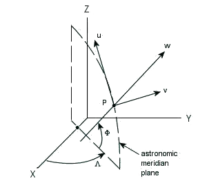
The other two coordinate systems we need are the local astronomic (LA) system and the local geodetic (LG) system. Both of these 3D systems have their origin at the station marker, where we make our measurements.
We will name the three axes of the LA system u, v, w (as shown in the diagram at the right), and those of the LG system x, y, z.
The LA system w-axis is coincident with the local gravity vector at the point P, and is positive upwards. The LA u-axis points to astronomic north, and the LA v-axis points to astronomic east to make a left-handed 3D Cartesian system.
The LG system is very similar to the LA system. The LG z-axis is coincident with the ellipsoidal normal at the station marker, and is positive upwards. The LG x-axis points to geodetic north, and the LG y-axis points to geodetic east.
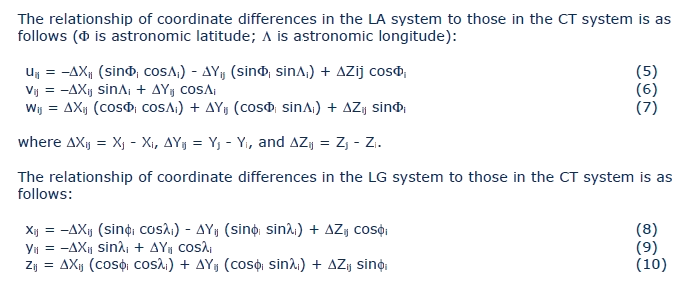
As you can see, all of the above equations are exact. Therefore we have the basis, in the above equations, to relate a measured quantity (e.g. a distance, an angle, a GPS vector, ISS coordinate differences, leveled height differences, etc.) to either the LG or LA coordinate differences between the stations involved in the measurement. We also have the exact mathematical relationship between either the LA or LG systems and the CT system.
The above equations form the basis from which all mathematical models used in GeoLab are derived. As an example of how the mathematical models are derived, let's consider a spatial distance measurement. The relationship between a spatial distance Sij from point i to point j, to the CT coordinates of the two stations is as follows:

and it's linearized version (required for the adjustment) is given by

Because we have the relationship between CT coordinate differences and those in either the LA or LG systems, we can now easily transform this observation equation to the LG or LA systems. All the information needed to do this has been given in this article. For the detailed development, please have a look at the report referenced above.
As can be seen, we do not need to make reductions to our measurements with approximate formulae at all. If you compare the observation equations in this exact method with the older 2D observation equations, you'll see that the 3D models are as simple as the older, less accurate models, especially when you consider all the approximate and involved reduction formulae we used to use.